CS 184 Final Report: Subsurface Scattering
Milestone ProposalAbstract
Subsurface scattering is the scattering of light under the surface of translucent materials. This allows for even more realistic physically based rendering (jade, marble, skin, etc.). The BSSRDF adds further dimensionality to the BRDF, as the ray exits from a different location. The authoritative paper this project was inspired by was Jensen et al. 2001 which develops a computationally feasible method to model ray paths beneath the surface.
Technical Approach
BSSRDF Model
\( S(x_i, \vec{w_i}; x_o, \vec{w_o}) = S_d(x_i, \vec{w_i}; x_o, \vec{w_o}) + S^{(1)}(x_i, \vec{w_i}; x_o, \vec{w_o}) \)
Diffusion
\( S_d(x_i, \vec{w_i}; x_o, \vec{w_o}) = \frac{1}{\pi}F_t(\eta, \vec{w_i})R_d(\left\lVert x_i-x_o\right\rVert)F_t(\eta,\vec{w_o}) \)
Vector3D BSSRDF::diffusion_term(Vector3D xi, Vector3D wi, Vector3D xo, Vector3D wo) {
    Vector3D e(exp(1));
    double F = diffuse_fresnel_reflectance();
    double A = (1 + F) / (1 - F);
    double r = (xi - xo).norm();
    Vector3D extinction = scattering / 100 + absorption / 100; // sigma t
    Vector3D effective_extinction = vec_sqrt(3 * (extinction / 100) * (absorption / 100));
    Vector3D reduced_albedo = scattering / (scattering + absorption);
    Vector3D D = 1 / (3 * extinction * reduced_albedo);
    Vector3D z_r = 1 / reduced_albedo;
    Vector3D z_v = z_r + 4 * A * D;
    Vector3D R_d = (reduced_albedo / (4 * PI)) *
        ((effective_extinction * z_r + Vector3D(1)) * vec_pow(e, -effective_extinction * z_r) / (extinction * vec_pow(z_r, Vector3D(3))) +
        z_v *(effective_extinction * z_v + Vector3D(1)) * vec_pow(e, -effective_extinction * z_v) / (extinction * vec_pow(z_v, Vector3D(3))));
    return (1 / PI) * fresnel_transmittance(1 / eta, wo) * R_d * fresnel_transmittance(eta, wi);
}
Single Scattering
\( L_o^{(1)}(x_o, \vec{w_o}) = \int_A\int_{2\pi}S^{(1)}(x_i, \vec{w_i}; x_o, \vec{w_o})L_i(x_i,\vec{w_i})(\vec{n}\cdot\vec{w_i})dw_idA(x_i) \)
Vector3D BSSRDF::single_scattering_term(Vector3D xi, Vector3D wi, Vector3D xo, Vector3D wo) {
    Vector3D extinction = scattering + absorption;
    Vector3D effective_extinction = vec_sqrt(3 * extinction * absorption);
    double si = (xi - xo).norm();
    double LdotNi = fabs(wi.z);
    double sp_i = si * LdotNi / sqrt(1 - (1.0 / eta) * (1.0 / eta) * (1 - LdotNi * LdotNi));
    double phase = 1.0;

    double G = fabs(wo.z) / fabs(wi.z);
    Vector3D sigma_tc = extinction + G * extinction;
    return PI * scattering * vec_pow(Vector3D(exp(1)), -sp_i * extinction) / sigma_tc * phase * fresnel_transmittance(eta, wi) * fresnel_transmittance(1 / eta, wo);
}
For the light transmission we leveraged the derivations from the Jensen paper. The two terms that make up the BSSRDF model were the diffusion and single scattering terms, which take in not only the intersection point and directions, but also the exiting intersection point.
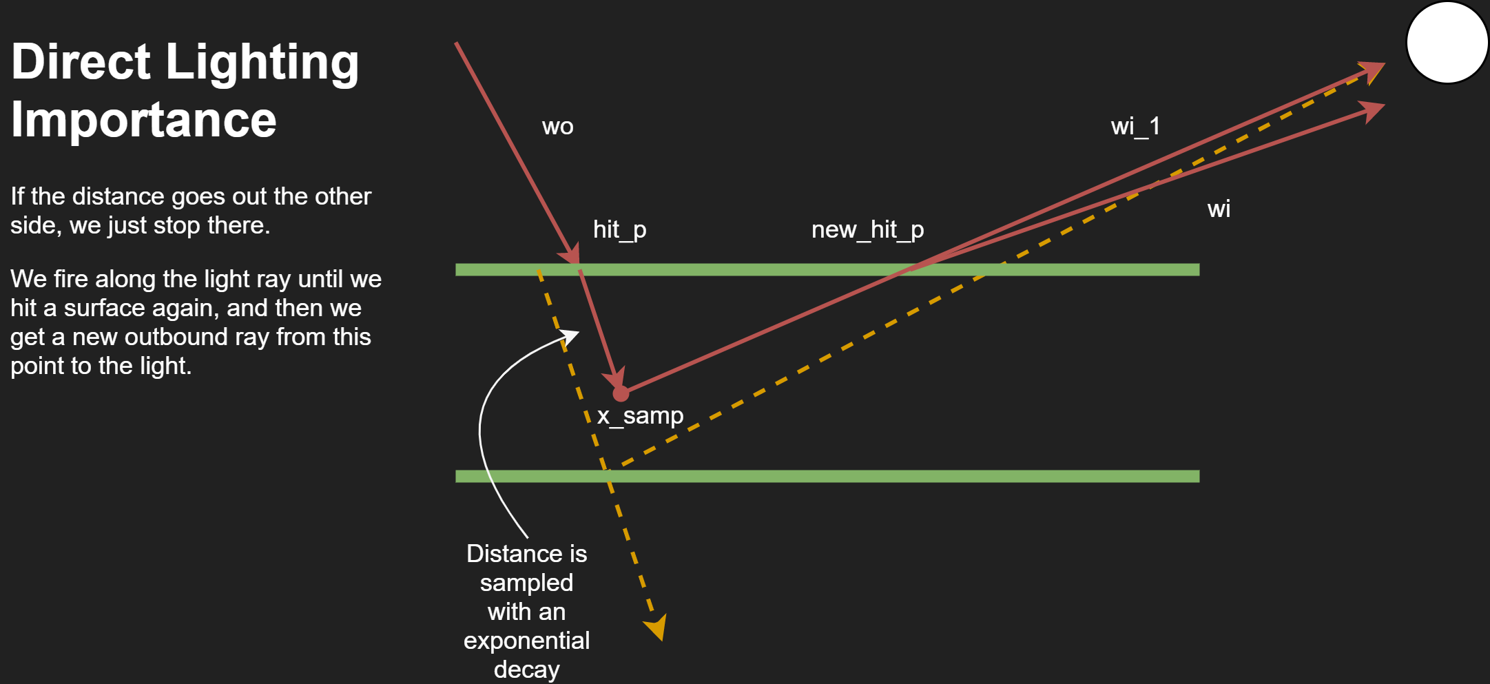
The majority of the effect comes from importance sampling lighting illumination and single scattering. The diagram above shows a high level overview of our implementation. We shoot a ray further into the material based on an exponential decay and material parameters, and from the inner point we sample a point to the light. The total distance traveled in the material is used to attenuate the light. This is highly simplified as the total equation captures the Fresnel terms for entering and exiting the materials and some other subtle factors.
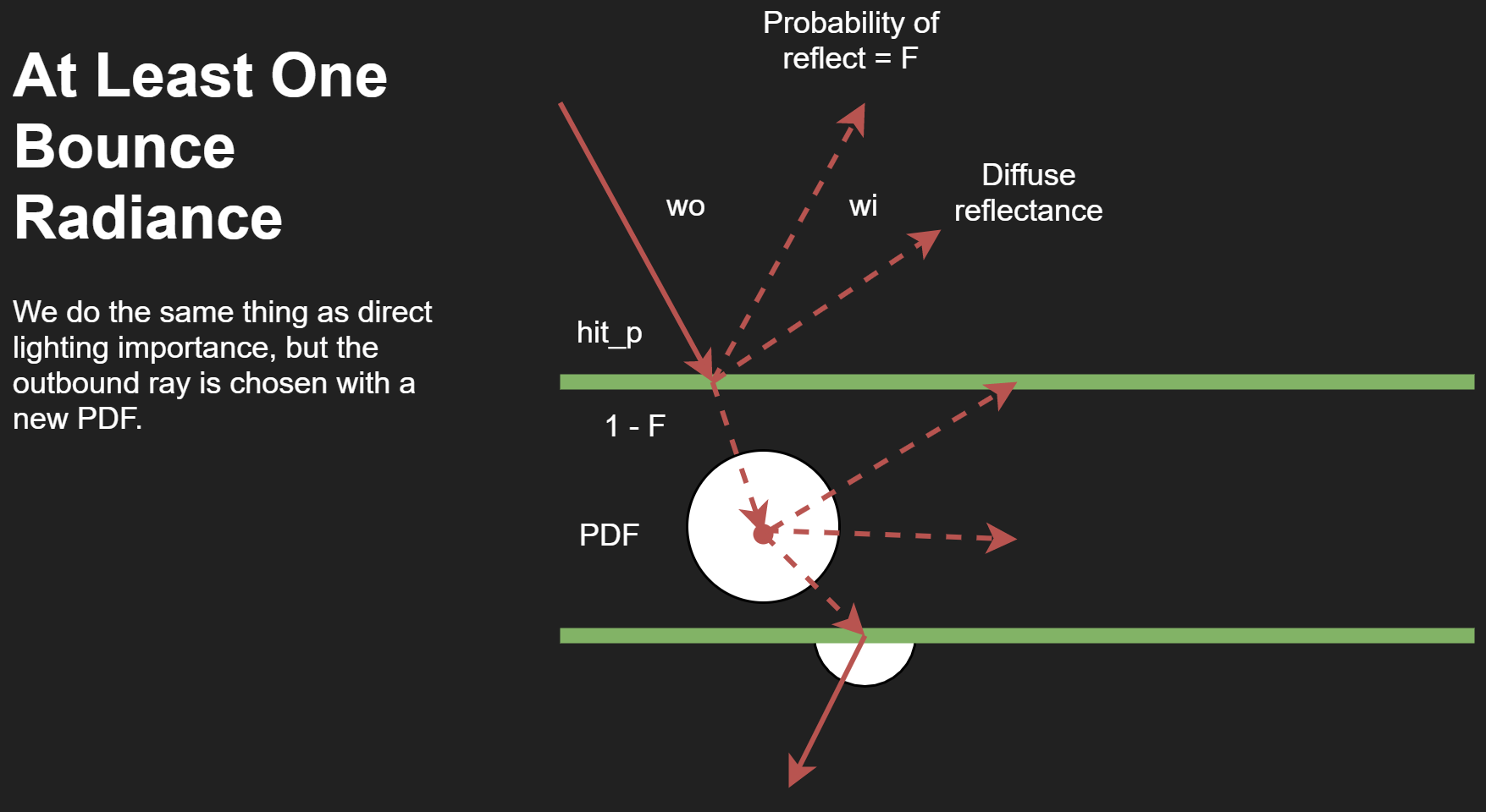
For multi-bounce lighting, the ray can either pass into the material for subsurface scattering, bounce off in a diffuse manner, or be a perfect reflection. For rays that enter, we sample the distance in just like before, but now choose a new ray direction to exit from. Then we follow this ray to a new point on the surface and can continue bouncing as normal outside.
Relevant Files:
collada.cppbsdf.hadvanced_bsdf.cpppathtracer.cpp
For the code itself we first had to modify the parser to accept customized dae files that pass in our needed parameters. Then, we implemented a naive approximation of the BSSRDF and the BSSRDF itself. This is where we applied the formulaic derivations from the paper for the actual values of light transmission factor. The interface for a BSDF had to be modified to support a higher dimensional function. Finally, we had to make significant changes to the pathtracer itself to account for the ray penetrating the surface of the material and usage of our BSSRDF.
Deviations from the paper include slight inaccuracies in the use of the PDF for a now biased Monte Carlo integration, averaging some material parameters in one part of the flow (average scattering) across all RGB channels instead of handling it entirely per channel leading to some color imbalance, and manually tuned diffuse reflection.
The magnitude of the ray shot into the material was dependent on the parameters, which causes drastically different visual outputs. We had to scale the parameters which can be considered as having the object itself be different sizes in real life. Additionally, we were initially getting results that were too bright, with some ‘caustic’-like effects. We had to clamp the values which fixed most of the visual issues. When even one part of the formula has a value inverted, we can get results that look very interesting, as seen in our milestone results.
Overall, we have deepened our understanding of the BRDF and how it is extended to a BSSRDF to support subsurface scattering. The initial pathtracing model in class served as a baseline to figure out how we can fire more rays beneath the surface of the object to add another dimensionality to our calculations. We learned more about how the pathtracer program from class worked as we had to make significant changes to support subsurface scattering.
Additionally, we learned how difficult it is to discern physical correctness of the model based on the initial visual appearance. It took inspection of very specific parts of a model to see slight inaccuracies with lighting. Additionally, we purposely approximated and clamped parts of the formulas used and that also revealed how the visual appearance still looked somewhat physically accurate. While in the end we could not solve every physically inaccurate issue with our renderer, we still ended up with a very satisfying result.
Results
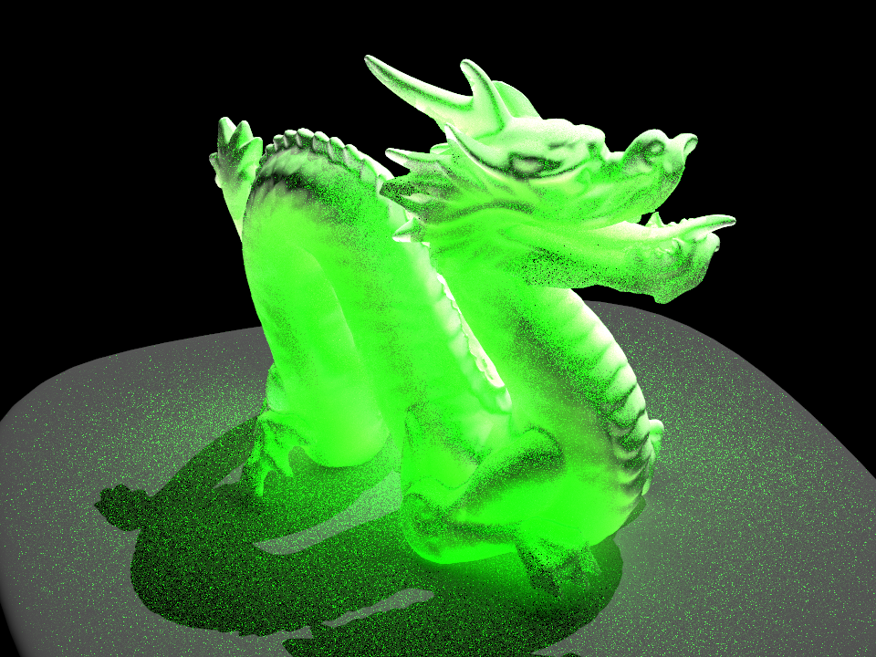
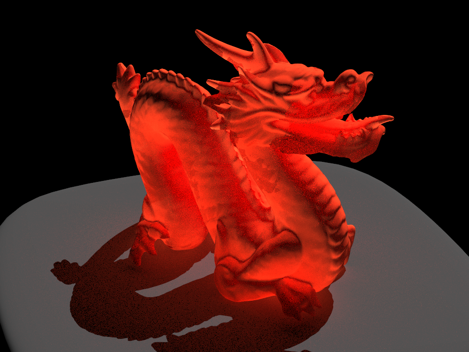
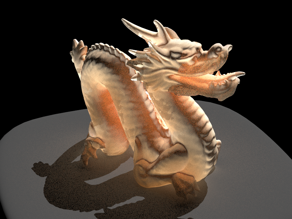
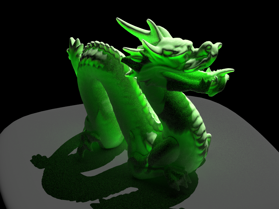
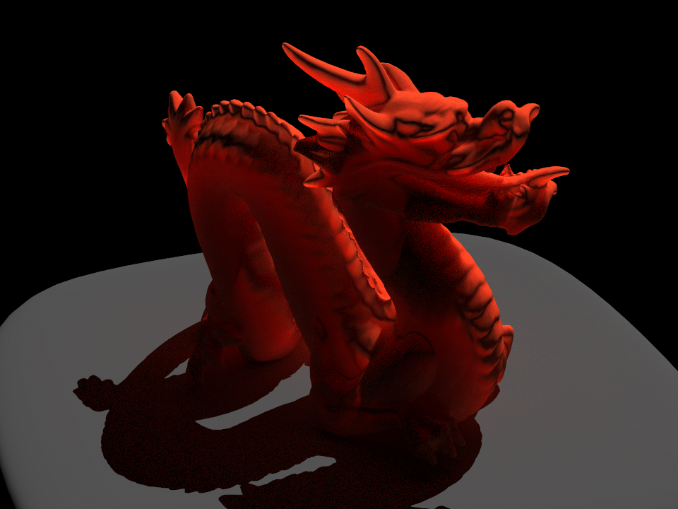
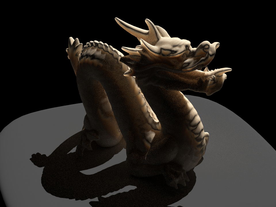
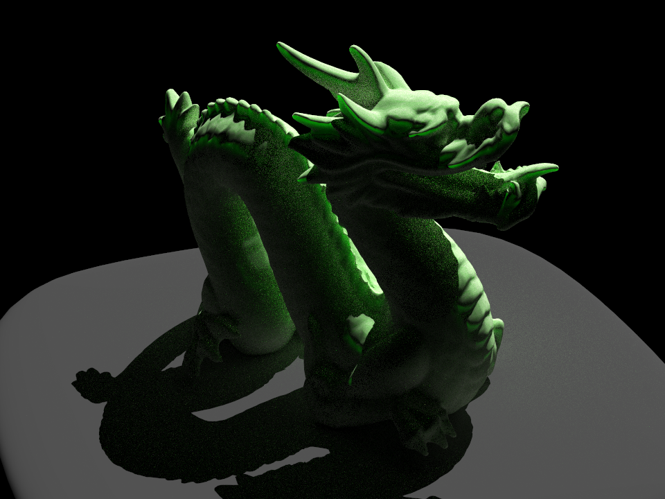
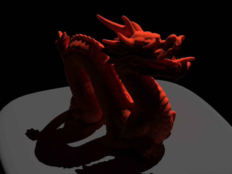
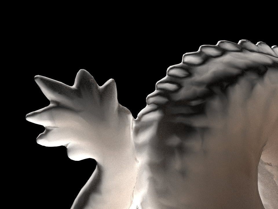
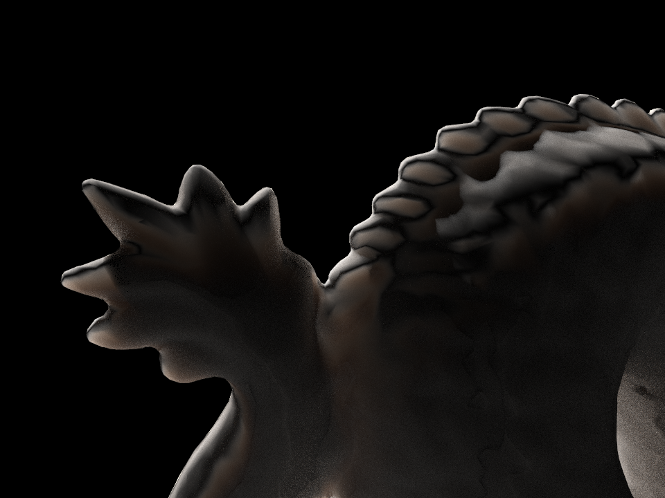
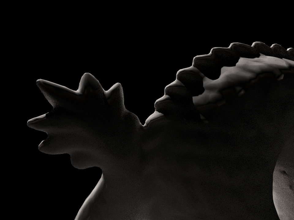
Each scene had a single point light source in front of the dragon. For the following renderings, the camera is positioned behind the dragon to show the translucent effect of subsurface scattering.
Scale factor refers to scaling the model size by an integer factor. i.e. A scale factor of 10 would result in a dragon 10 times as large in real life.
| Scale Factor | "Marble" | "Jade" | "Ketchup" | "Skin" |
|---|---|---|---|---|
| 10 | 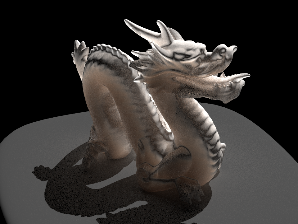 |
 |
 |
 |
| 10 | 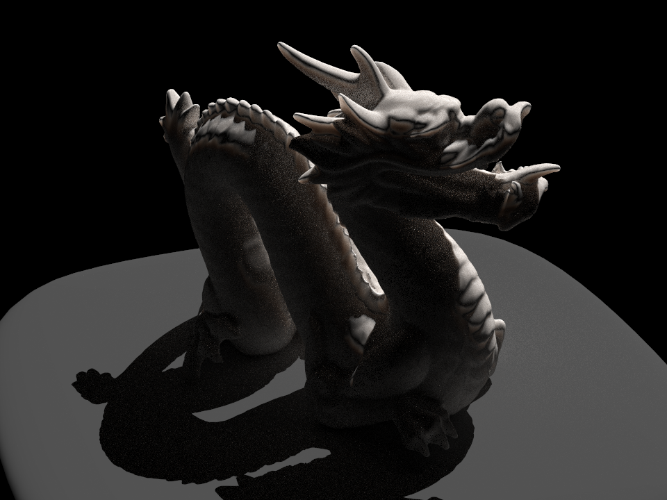 |
 |
 |
 |
| 1000 | 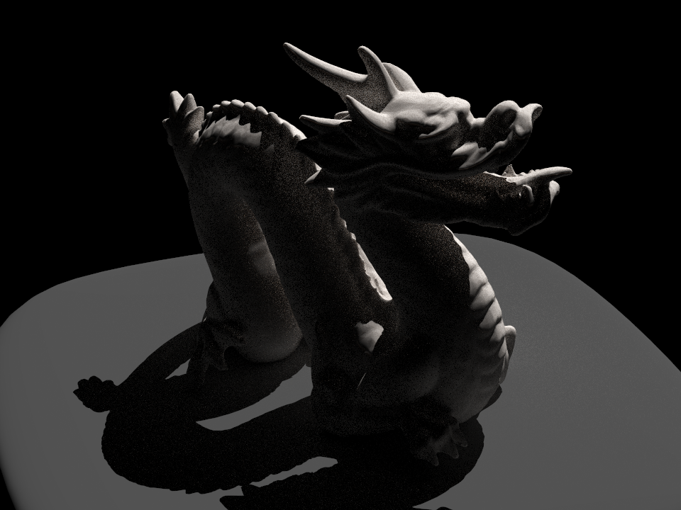 |
 |
 |
 |
The camera angle for these renderings was from the back of the dragon and focused in on the tail portion of the dragon.
References
- A Practical Model for Subsurface Light Transport
- Approximate Reflectance Profiles for Efficient Subsurface Scattering
- BSSRDF Importance Sampling
- A Layered, Heterogeneous Reflectance Model for Acquiring and Rendering Human Skin
- RenderMan, Theory and Practice
- Subsurface Scattering Using the Diffusion Equation
Contributions
- Andy: Worked on main renderer code, rendered animations.
- Kevin: Set up base framework for the BSSRDFs, worked on main renderer code.
- Jemmy: Worked on main renderer code, put up website.
- Jeffrey: Worked on main renderer code, made explanation diagrams.